Faster Generation of Quantile Quantile Plots with Large Samples

New and faster implementations for quantile quantile plots. The package also includes a function to prune data for quantile quantile plots. This can drastically reduce the running time for large samples, for 100 million samples, you can expect a factor 80X speedup.

fastqq

fastqq is intended for creating quantile-quantile plots. We provide faster alternatives to qqman::qq, stats::qqplot and stats::qqnorm. We also provide the function fastqq::drop_dense such that the user can extract the data to plot with ggplot.

For 100 million samples, we achieve 80X speedup compared to qqman::qq. This takes the running time from ~13.5 minutes down to less than 10 seconds.

Background

This package was originally intended to speedup the creation of QQ plots for genome wide association studies (GWAS). Then I decided to make it a general tool fro QQ style plots. For QQ plots, the user often plots tens to hundreds of millions of points. Creating scatter plots with so many points is usually not efficient since the graphics devices store all the data, such that the visualization can be rescaled or plotted in a vector graphics format (where again all the data is stored).

A better and faster approach in these cases is to note that many of the points are so close to each other that there is no value in including them in the plot. QQ style plots are usually a monotonically increasing sequence of points, so we can easily employ fast filtering to remove redundant points, that would otherwise not be visible in the final plot anyways.

See examples below.

Note that this package is inspired by the qqman package, which has now been archived. The interface to the qq function should be very similar, and fastqq::qq is a drop-in replacement for qqman::qq. I created this package since it could take more than 10 minutes to render a single plot with qqman::qq. This is also to save on memory and other resources, in particular time.

Installation

You can install the released version of fastqq from CRAN with:

install.packages("fastqq")

And the development version from GitHub with:

# install.packages("devtools")
devtools::install_github("gumeo/fastqq")

Example

The following is an example from very simple simulated data:

suppressPackageStartupMessages(library(fastqq))
set.seed(42)
p_simulated <- runif(1e5)
# Classic way to do this with qqman
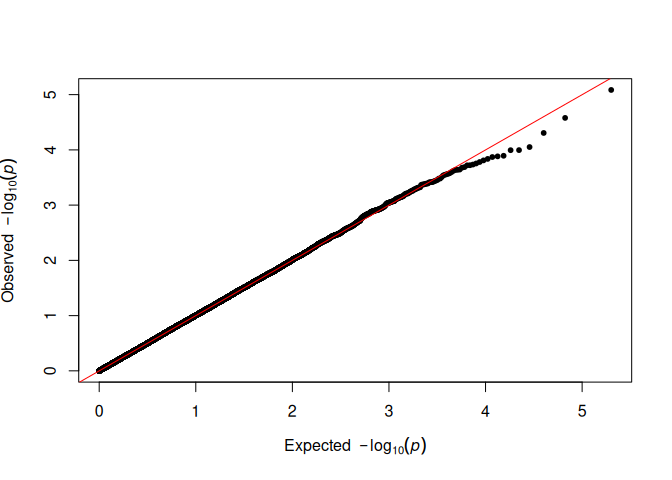
qqman::qq(p_simulated)

# Alternative
fastqq::qq(p_simulated)

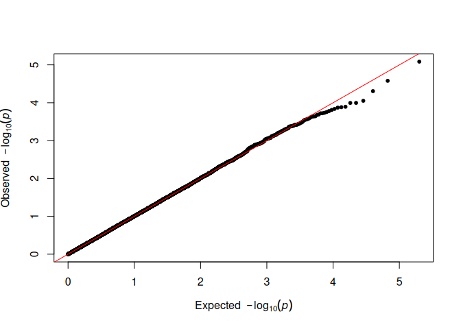
There is no visible difference, and the analysis can proceed as usual.

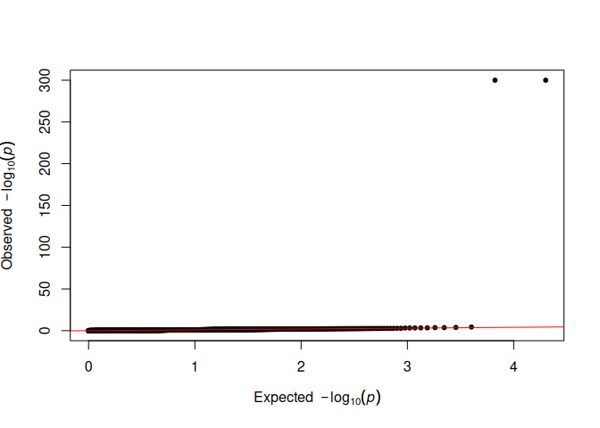
If some p-values are exactly zero (e.g. from software that reports underflowed results), use the zero_action parameter to substitute a small finite value:

pvec_with_zeros <- c(runif(1e4), 0, 0)
qq(pvec_with_zeros, zero_action = 1e-300)
#> Warning in qq(pvec_with_zeros, zero_action = 1e-300): 2 p-value(s) equal to
#> zero replaced with 1e-300.

We can compare the timings of creating the plots, with qqman.

set.seed(555)
N_test <- c(1e3,1e4,1e5,1e6)
time_method <- function(pkg_name, method){
  suppressPackageStartupMessages(library(pkg_name, 
                                         character.only=TRUE, quietly = TRUE))
  for(N in N_test){
    p_vec <- runif(n = N)
    print(paste0("Timing ", pkg_name, "::", method," with ", 
                 N, " points"))
    tictoc::tic()
    pdf(file = NULL) # Prevent the plots from appearing
    do.call(method, list(pvector=p_vec))
    dev.off()
    tictoc::toc()  
  }
}
N_test <- c(1e3,1e4,1e5,1e6,1e8)
time_method('fastqq','qq')
#> [1] "Timing fastqq::qq with 1000 points"
#> 0.028 sec elapsed
#> [1] "Timing fastqq::qq with 10000 points"
#> 0.02 sec elapsed
#> [1] "Timing fastqq::qq with 1e+05 points"
#> 0.049 sec elapsed
#> [1] "Timing fastqq::qq with 1e+06 points"
#> 0.414 sec elapsed
#> [1] "Timing fastqq::qq with 1e+08 points"
#> 48.603 sec elapsed
N_test <- c(1e3,1e4,1e5,1e6)
time_method('qqman','qq')
#> [1] "Timing qqman::qq with 1000 points"
#> 0.002 sec elapsed
#> [1] "Timing qqman::qq with 10000 points"
#> 0.02 sec elapsed
#> [1] "Timing qqman::qq with 1e+05 points"
#> 0.189 sec elapsed
#> [1] "Timing qqman::qq with 1e+06 points"
#> 1.989 sec elapsed

So we can expect around 25X speedup for a million points. For 100 million points (order of magnitude for modern GWAS), fastqq::qq takes 10 seconds on the same hardware as for the timings above, qqman::qq takes more than 13.78 minutes for 100 million points (80X speedup) and if one saves to a vector graphic output, all the data is stored, and the file size scales with the amount of points.

qqlog example

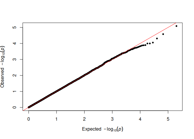
qqlog accepts pre-computed −log₁₀(p-values). This is useful when you have already transformed your p-values, or need full precision before plotting (e.g. values below .Machine$double.xmin computed in extended precision):

set.seed(42)
suppressPackageStartupMessages(library(fastqq))
pvec <- runif(1e5)
fastqq::qqlog(-log10(pvec))

qqchisq1 example

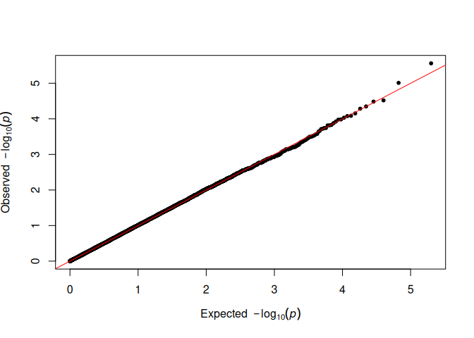
qqchisq1 accepts χ² test statistics and converts them to −log₁₀(p) assuming 1 degree of freedom. The conversion uses log-space arithmetic for numerical stability even for very large statistics:

set.seed(42)
suppressPackageStartupMessages(library(fastqq))
chisq_vals <- rchisq(1e5, df = 1)
fastqq::qqchisq1(chisq_vals)

Handling astronomically small p-values

A χ² value of ~2303 (df=1) corresponds to p ≈ 10⁻⁵⁰⁰, which is far below R’s double-precision floor of .Machine$double.xmin ≈ 2.2×10⁻³⁰⁸. Naive computation underflows to zero, making the point invisible to any method that works on the raw p-value scale:

suppressPackageStartupMessages(library(fastqq))

extreme_chisq <- 2303  # p ≈ 10^-500

# Naive approach: p-value underflows to 0, point is lost
cat("Naive p-value:          ", pchisq(extreme_chisq, 1, lower.tail = FALSE), "\n")
#> Naive p-value:           0

# Log-space gives the correct -log10(p) even for such extreme values
cat("-log10(p) via log-space:",
    -pchisq(extreme_chisq, 1, lower.tail = FALSE, log.p = TRUE) / log(10), "\n")
#> -log10(p) via log-space: 501.8695

# qqchisq1 uses log-space internally, so the extreme point appears correctly
set.seed(42)
chisq_vals <- c(rchisq(1e4, df = 1), extreme_chisq)
fastqq::qqchisq1(chisq_vals)

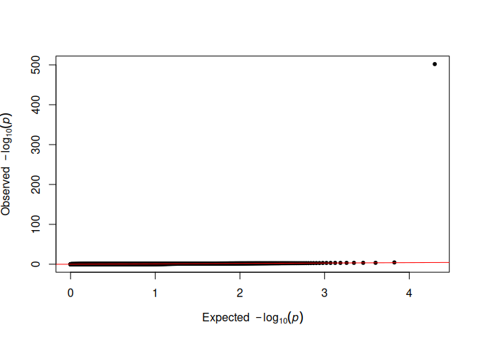
The extreme point appears at the top of the plot (~500 on the y-axis) without any special handling required from the user.

qqnorm example

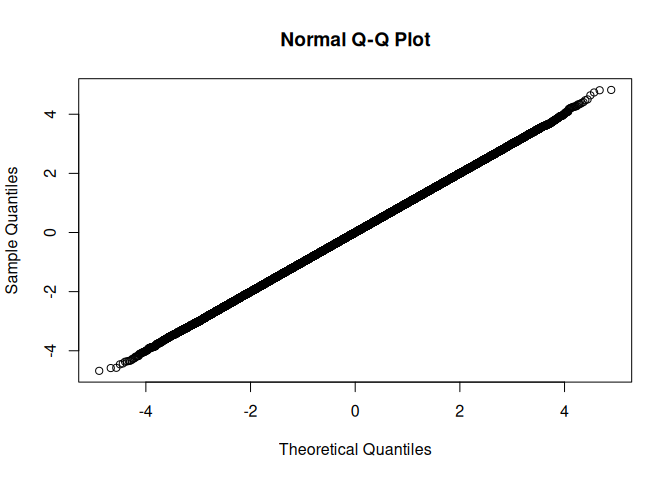
We can use qqnorm just like from stats::qqnorm. The only difference is in the output, we return sorted output, and exclude NAs.

set.seed(42)
suppressPackageStartupMessages(library(fastqq))
fastqq::qqnorm(rnorm(1e6))

qqplot example

set.seed(42)
suppressPackageStartupMessages(library(fastqq))
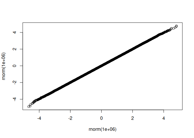
fastqq::qqplot(rnorm(1e6),rnorm(1e6))

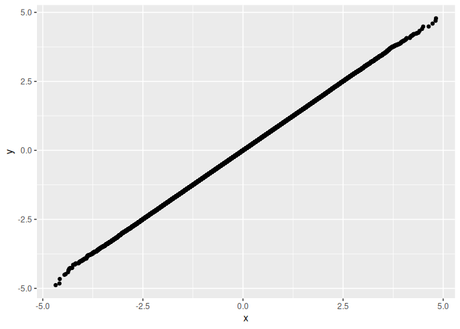
drop_dense and plot with ggplot example

set.seed(42)
suppressPackageStartupMessages(library(fastqq))
suppressPackageStartupMessages(library(ggplot2))
x <- rnorm(1e6)
y <- rnorm(1e6)
df <- fastqq::drop_dense(x, y)

ggplot(df, aes(x=x,y=y)) + geom_point()

Note on other efforts

After I created this, I have found several sources, that aim at something similar, usually also a manhattan plot (I am probably also missing other packages):

• fastman package. Uses scattermore, so the plotting is very fast. This package is not currently (31/07/2021) on CRAN.
• ramwas package. Has not been maintained in 2 years and is on bioconductor. This package is aimed for Fast Methylome-Wide Association Study Pipeline for Enrichment Platforms and the ramwas::qqPlotFast function is just a minor part of the package. It

Here are also some projects on CRAN, where the plotting is similar to qqman::qq, and is not improved for speed.

• gwaRs package. Focuses on using ggplot.
• manhplot package. This is a pretty ambitious project, with a good publication. Again, the main focus is on the manhattan plot.
• qqman package. Probably one of the main inspiration for most of the other packages.
• CMplot package. Great circular manhattan plot.