Echo State Networks for Time Series Modeling and Forecasting

Provides a lightweight implementation of functions and methods for fast and fully automatic time series modeling and forecasting using Echo State Networks (ESNs).

echos

The echos package provides a comprehensive set of functions and methods for modeling and forecasting univariate time series using Echo State Networks (ESNs). It offers two alternative approaches:

Base R interface: Functions for modeling and forecasting time series using numeric vectors, allowing for straightforward integration with existing R workflows.
Tidy interface: A seamless integration with the fable framework based on tsibble, enabling tidy time series forecasting and model evaluation. This interface leverages the fabletools package, providing a consistent and streamlined workflow for model development, evaluation, and visualization.

The package features a lightweight implementation that enables fast and automatic model training and forecasting using ESNs. You can quickly and easily build accurate ESN models without requiring extensive hyperparameter tuning or manual configuration.

Model specification

echos implements Echo State Networks with a fixed randomly initialized reservoir and a ridge-regression readout. The input and reservoir weights are generated once and kept fixed, while only the readout layer is estimated.

The main ESN hyperparameters are the reservoir size (n_states), leakage rate (alpha), spectral radius (rho), reservoir density (density), input scaling (scale_inputs, scale_win, scale_wres), and the ridge regularization range (lambda). These parameters control the memory, stability, complexity, and regularization of the model.

By default, train_esn() automatically determines the number of differences, constructs the reservoir, evaluates candidate ridge readout models, and selects the final readout using an information criterion. For explicit grid-based tuning of alpha, rho, and tau, use tune_esn().

Installation

You can install the stable version from CRAN:

install.packages("echos")

You can install the development version from GitHub:

# install.packages("devtools")
devtools::install_github("ahaeusser/echos")

Base R

library(echos)

# Forecast horizon
n_ahead <- 12 # forecast horizon
# Number of observations
n_obs <- length(AirPassengers)
# Number of observations for training
n_train <- n_obs - n_ahead

# Prepare train and test data
xtrain <- AirPassengers[(1:n_train)]
xtest <- AirPassengers[((n_train+1):n_obs)]

# Train and forecast ESN model
xmodel <- train_esn(y = xtrain)
xfcst <- forecast_esn(xmodel, n_ahead = n_ahead)

# Plot result
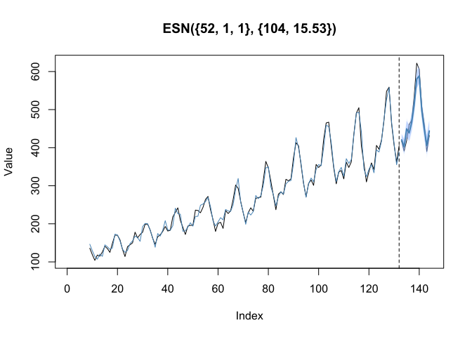
plot(xfcst, test = xtest)

Tidy R

library(echos)
library(tidyverse)
library(tsibble)
library(fable)

# Prepare train data
train_frame <- m4_monthly_subset %>%
  filter(series %in% c("M21655", "M2717"))

# Train and forecast ESN model
train_frame %>%
  model(
    "ESN" = ESN(value),
    "ARIMA" = ARIMA(value)
    ) %>%
  forecast(h = 18) %>%
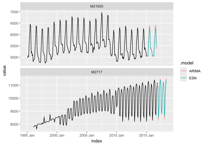
  autoplot(train_frame, level = NULL)

References

Häußer, A. (2026). Echo State Networks for Time Series Forecasting: Hyperparameter Sweep and Benchmarking. arXiv preprint arXiv:2602.03912. https://arxiv.org/abs/2602.03912
Jaeger, H. (2001). The “echo state” approach to analysing and training recurrent neural networks (with an erratum note). Bonn, Germany: German National Research Center for Information Technology (GMD), Technical Report 148(34):13.
Jaeger, H. (2002). Tutorial on training recurrent neural networks, covering BPPT, RTRL, EKF and the “echo state network” approach.
Lukosevicius, M. (2012). A practical guide to applying echo state networks. In Neural Networks: Tricks of the Trade (2nd ed.), pp. 659–686. Springer.
Lukosevicius, M., & Jaeger, H. (2009). Reservoir computing approaches to recurrent neural network training. Computer Science Review, 3(3), 127–149.