Density Ratio Estimation

Density ratio estimation. The estimated density ratio function can be used in many applications such as anomaly detection, change-point detection, covariate shift adaptation. The implemented methods are uLSIF (Hido et al. (2011) ), RuLSIF (Yamada et al. (2011) ), and KLIEP (Sugiyama et al. (2007) ).

An R Package for Density Ratio Estimation

Koji MAKIYAMA (@hoxo-m)

1. Overview

Density ratio estimation is described as follows: for given two data samples x1 and x2 from unknown distributions p(x) and q(x) respectively, estimate w(x) = p(x) / q(x), where x1 and x2 are d-dimensional real numbers.

The estimated density ratio function w(x) can be used in many applications such as anomaly detection [Hido et al. 2011], change-point detection [Liu et al. 2013], and covariate shift adaptation [Sugiyama et al. 2007]. Other useful applications about density ratio estimation were summarized by [Sugiyama et al. 2012].

The package densratio provides a function densratio() that returns an object with a method to estimate density ratio as compute_density_ratio().

For example,

set.seed(3)
x1 <- rnorm(200, mean = 1, sd = 1/8)
x2 <- rnorm(200, mean = 1, sd = 1/2)

library(densratio)
densratio_obj <- densratio(x1, x2)

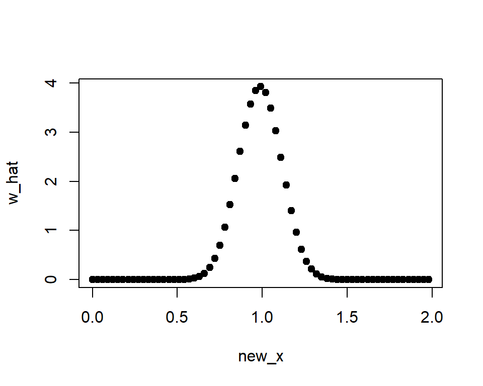
The densratio object has a function compute_density_ratio() that can compute the estimated density ratio w_hat(x) for any d-dimensional input x (now d=1).

new_x <- seq(0, 2, by = 0.03)
w_hat <- densratio_obj$compute_density_ratio(new_x)

plot(new_x, w_hat, pch=19)

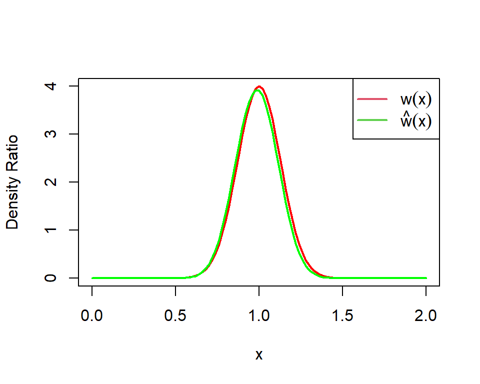
In this case, the true density ratio w(x) = p(x)/q(x) = Norm(1, 1/8) / Norm(1, 1/2) is known. So we can compare w(x) with the estimated density ratio w-hat(x).

true_density_ratio <- function(x) dnorm(x, 1, 1/8) / dnorm(x, 1, 1/2)

plot(true_density_ratio, xlim=c(0, 2), lwd=2, col="red", xlab = "x", ylab = "Density Ratio")
plot(densratio_obj$compute_density_ratio, xlim=c(0, 2), lwd=2, col="green", add=TRUE)
legend("topright", legend=c(expression(w(x)), expression(hat(w)(x))), col=2:3, lty=1, lwd=2, pch=NA)

2. Installation

You can install the densratio package from CRAN.

install.packages("densratio")

You can also install the package from GitHub.

install.packages("remotes") # if you have not installed "remotes" package
remotes::install_github("hoxo-m/densratio")

The source code for densratio package is available on GitHub at

• https://github.com/hoxo-m/densratio.

3. Details

3.1 Basics

The package provides densratio(). The function returns an object that has a function to compute estimated density ratio.

For data samples x1 and x2,

set.seed(3)
x1 <- rnorm(200, mean = 1, sd = 1/8)
x2 <- rnorm(200, mean = 1, sd = 1/2)

library(densratio)
densratio_obj <- densratio(x1, x2)

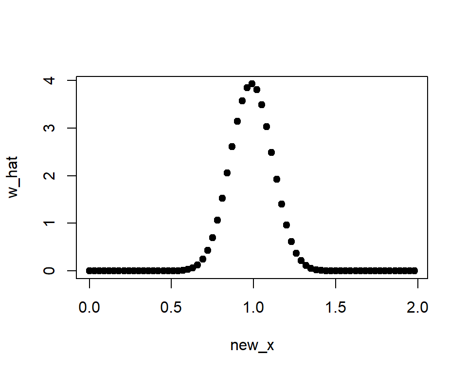
In this case, densratio_obj$compute_density_ratio() can compute estimated density ratio.

new_x <- seq(0, 2, by = 0.03)
w_hat <- densratio_obj$compute_density_ratio(new_x)

plot(new_x, w_hat, pch=19)

3.2 Methods

densratio() has method argument that you can pass "uLSIF", "RuLSIF", or "KLIEP".

• uLSIF (unconstrained Least-Squares Importance Fitting) is the default method. This algorithm estimates density ratio by minimizing the squared loss. You can find more information in [Kanamori et al. 2009] and [Hido et al. 2011].
• RuLSIF (Relative unconstrained Least-Squares Importance Fitting). This algorithm estimates relative density ratio by minimizing the squared loss. You can find more information in [Yamada et al. 2011] and [Liu et al. 2013].
• KLIEP (Kullback-Leibler Importance Estimation Procedure). This algorithm estimates density ratio by minimizing Kullback-Leibler divergence. You can find more information in [Sugiyama et al. 2007].

The methods assume that density ratios are represented by linear model:

• w(x) = theta_1 * K(x, c_1) + theta_2 * K(x, c_2) + ... + theta_b * K(x, c_b)

where

• K(x, c) = exp(-||x - c||^2 / (2 * sigma^2))

is the Gaussian (RBF) kernel.

densratio() performs the following:

• Decides kernel parameter sigma by cross-validation,
• Optimizes the kernel weights theta (in other words, find the optimal coefficients of the linear model), and
• The parameters sigma and theta are saved into densratio object, and are used when to compute density ratio in the call compute_density_ratio().

3.3 Result and Arguments

densratio() outputs the result like as follows:

#> 
#> Call:
#> densratio(x1 = x1, x2 = x2, method = "uLSIF")
#> 
#> Kernel Information:
#>   Kernel type:  Gaussian 
#>   Number of kernels:  100 
#>   Bandwidth (sigma):  0.1 
#>   Centers:  num [1:100, 1] 0.907 1.093 1.18 1.136 1.046 ...
#> 
#> Kernel Weights:
#>   num [1:100] 0.067455 0.040045 0.000459 0.016849 0.067084 ...
#> 
#> Regularization Parameter (lambda):  1 
#> 
#> Function to Estimate Density Ratio:
#>   compute_density_ratio()

• Kernel type is fixed as Gaussian.
• Number of kernels is the number of kernels in the linear model. You can change by setting kernel_num argument. In default, kernel_num = 100.
• Bandwidth (sigma) is the Gaussian kernel bandwidth. In default, sigma = "auto", the algorithm automatically select an optimal value by cross validation. If you set sigma a number, that will be used. If you set sigma a numeric vector, the algorithm select an optimal value in them by cross validation.
• Centers are centers of Gaussian kernels in the linear model. These are selected at random from the data sample x1 underlying a numerator distribution p(x). You can find the whole values in result$kernel_info$centers.
• Kernel Weights are theta parameters in the linear kernel model. You can find these values in result$kernel_weights.
• Function to Estimate Density Ratio is named compute_density_ratio().

4. Multi Dimensional Data Samples

So far, the input data samples x1 and x2 were one dimensional. densratio() allows to input multidimensional data samples as matrix, as long as their dimensions are the same.

For example,

library(densratio)
library(mvtnorm)

set.seed(3)
x1 <- rmvnorm(300, mean = c(1, 1), sigma = diag(1/8, 2))
x2 <- rmvnorm(300, mean = c(1, 1), sigma = diag(1/2, 2))

densratio_obj_2d <- densratio(x1, x2)
densratio_obj_2d
#> 
#> Call:
#> densratio(x1 = x1, x2 = x2, method = "uLSIF")
#> 
#> Kernel Information:
#>   Kernel type:  Gaussian 
#>   Number of kernels:  100 
#>   Bandwidth (sigma):  0.316 
#>   Centers:  num [1:100, 1:2] 1.257 0.758 1.122 1.3 1.386 ...
#> 
#> Kernel Weights:
#>   num [1:100] 0.0756 0.0986 0.059 0.0797 0.0421 ...
#> 
#> Regularization Parameter (lambda):  0.3162278 
#> 
#> Function to Estimate Density Ratio:
#>   compute_density_ratio()

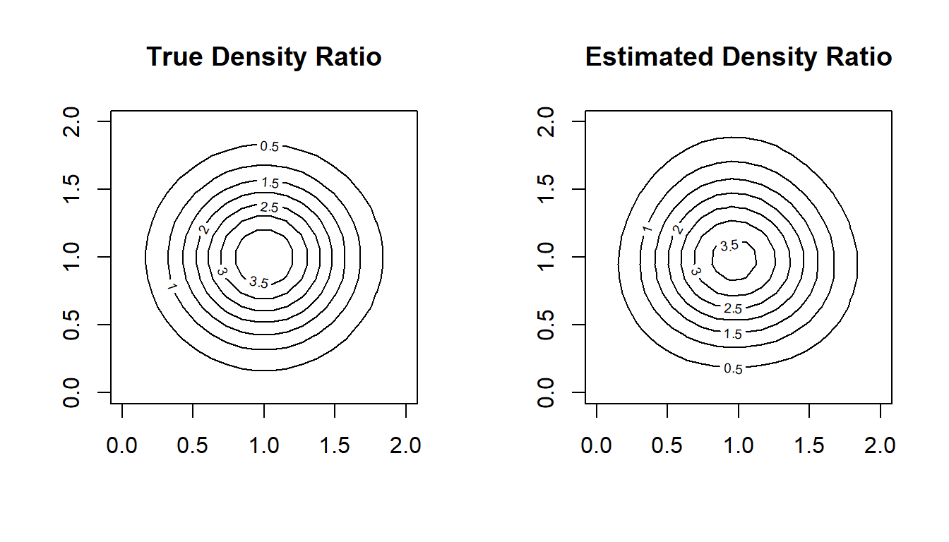
In this case, as well, we can compare the true density ratio with the estimated density ratio.

true_density_ratio <- function(x) {
  dmvnorm(x, mean = c(1, 1), sigma = diag(1/8, 2)) /
    dmvnorm(x, mean = c(1, 1), sigma = diag(1/2, 2))
}

N <- 20
range <- seq(0, 2, length.out = N)
input <- expand.grid(range, range)
w_true <- matrix(true_density_ratio(input), nrow = N)
w_hat <- matrix(densratio_obj_2d$compute_density_ratio(input), nrow = N)

par(mfrow = c(1, 2))
contour(range, range, w_true, main = "True Density Ratio")
contour(range, range, w_hat, main = "Estimated Density Ratio")

5. Used in research

The densratio package has been used in several research papers, including:

• Fricke, K.R., & Herzberg, P.Y. (2019). Know your big data: De-biasing subsamples of large datasets for personality research using importance sampling and kNN matching.
• Chen, M.F., Goel, K., Sohoni, N.S., Poms, F., Fatahalian, K., & R’e, C. (2021). Mandoline: Model Evaluation under Distribution Shift. International Conference on Machine Learning.
• Evans, C., & G’Sell, M. (2024). Sequential label shift detection in classification data: An application to dengue fever. PLOS ONE, 19.
• Chakraborty, A., Huan, X., & Catanach, T.A. (2024). A Likelihood-Free Approach to Goal-Oriented Bayesian Optimal Experimental Design.
• Awaya, N., Xu, Y., & Ma, L. (2025). Two-sample comparison through additive tree models for density ratios.

6. Related work

• A Python Package for Density Ratio Estimation
  • https://pypi.org/project/densratio/
• APPEstimation: Adjusted Prediction Model Performance Estimation
  • https://cran.r-project.org/package=APPEstimation

References

• Hido, S., Y. Tsuboi, H. Kashima, M. Sugiyama, and T. Kanamori. Statistical outlier detection using direct density ratio estimation. Knowledge and Information Systems, 2011.
• Kanamori, T., S. Hido, and M. Sugiyama. A least-squares approach to direct importance estimation. Journal of Machine Learning Research, 2009.
• Liu, S., M. Yamada, N. Collier, M. Sugiyama. Change-point detection in time-series data by relative density-ratio estimation. Neural Net, 2013
• Sugiyama, M., S. Nakajima, H. Kashima, P. von Bünau, and M. Kawanabe. Direct importance estimation with model selection and its application to covariate shift adaptation. NIPS 2007.
• Sugiyama, M., T. Suzuki, and T. Kanamori. Density ratio estimation in machine learning. Cambridge University Press, 2012.
• Yamada, M., T. Suzuki, T. Kanamori, H. Hachiya, and M. Sugiyama. Relative density-ratio estimation for robust distribution comparison. NIPS 2011.