aplms
Additive Partial Linear Models with Symmetric Autoregressive Errors
Set of tools for fitting the additive partial linear models with symmetric autoregressive errors of order p, or APLMS-AR(p). This setup enables the modeling of a time series response variable using linear and nonlinear structures of a set of explanatory variables, with nonparametric components approximated by natural cubic splines or P-splines. It also accounts for autoregressive error terms with distributions that have lighter or heavier tails than the normal distribution. The package includes various error distributions, such as normal, generalized normal, Student's t, generalized Student's t, power-exponential, and Cauchy distributions. Chou-Chen, S.W., Oliveira, R.A., Raicher, I., Gilberto A. Paula (2024)
aplms
The goal of aplms is fitting Additive partial linear models with
symmetric autoregressive errors (APLMS), proposed by Chou-Chen et al.,
(2024). This framework
models a time series response variable using both linear and nonlinear
structures of a set of explanatory variables, with the nonparametric
components approximated by natural cubic splines or P-splines. It also
accounts for autoregressive error terms with distributions that have
lighter or heavier tails than the normal distribution.
Installation
You can install the package with:
install.packages("aplms")
or the development version of aplms from GitHub with:
# install.packages("devtools")
devtools::install_github("shuwei325/aplms")
Model
The details of the model and its assumptions are given in Chou-Chen et al., (2024).
Example
This package provides two datasets to illustrate the model fitting procedure. To load the package:
library(aplms)
1. Global annual mean surface air temperature
The first dataset temperature:
data(temperature)

# Create dataframe object to fit the model
datos = data.frame(temperature,time=1:length(temperature))

mod1<-aplms::aplms(temperature ~ 1,
                   npc=c("time"), basis=c("cr"),Knot=c(60),
                   data=datos,family=Powerexp(k=0.3),p=1,
                   control = list(tol = 0.001,
                                  algorithm1 = c("P-GAM"),
                                  algorithm2 = c("BFGS"),
                                  Maxiter1 = 20,
                                  Maxiter2 = 25),
                   lam=c(10))
summary(mod1)
#>  ---------------------------------------------------------------
#>  Additive partial linear models with symmetric errors
#>  ---------------------------------------------------------------
#>  Sample size:  142
#>  -------------------------- Model ---------------------------
#>
#> aplms::aplms(formula = temperature ~ 1, npc = c("time"), basis = c("cr"),
#>     Knot = c(60), data = datos, family = Powerexp(k = 0.3), p = 1,
#>     control = list(tol = 0.001, algorithm1 = c("P-GAM"), algorithm2 = c("BFGS"),
#>         Maxiter1 = 20, Maxiter2 = 25), lam = c(10))
#>
#>  ------------------- Parametric component -------------------
#>
#>           Estimate Std. Error t value  Pr(>|t|)
#> intercept 0.056619     0.0041 13.8905 < 2.2e-16 ***
#>
#>  ----------------- Non-parametric component ------------------
#>
#>          Wald       df    Pr(>.)
#> time 7589.838   58.583 < 2.2e-16 ***
#>
#>  --------------- Autoregressive and Scale parameter ----------------
#>
#>        Estimate Std. Error    Wald  Pr(>|t|)
#> phi   0.0022992     0.0003  7.3902 1.242e-11 ***
#> rho1 -0.2571215     0.0662 -3.8866 0.0001568 ***
#>
#>
#> ------ Penalized Log-likelihood and Information criterion------
#>
#>  Log-lik:  200.07
#>  AIC    :  -276.97
#>  AICc   :  -274.46
#>  BIC    :  -94.94
#>  GCV    :  0.01
#>
#>  --------------------------------------------------------------------
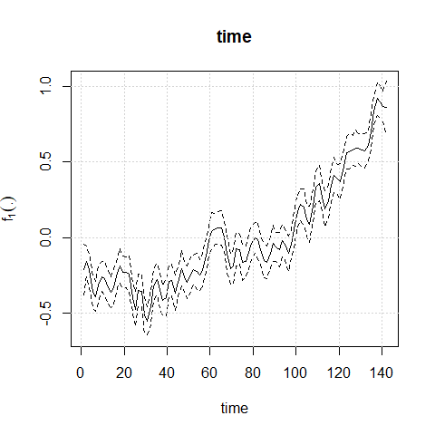
plot(mod1)
To perform diagnostic and influence analyses, execute:
aplms.diag.plot(mod1)
influenceplot.aplms(mod1,  perturbation = c("case-weight"))
2. Respiratory diseases
The second dataset hospitalization:
data(hospitalization)

mod2<-aplms::aplms(formula = y ~
              MP10_avg + NO_avg + O3_avg + TEMP_min + ampl_max + RH_max,
            npc=c("tdate","epi.week"), basis=c("cr","cc"),Knot=c(60,12),
            data=hospitalization,family=Powerexp(k=0.3),p=3,
            control = list(tol = 0.001,
                           algorithm1 = c("P-GAM"),
                           algorithm2 = c("BFGS"),
                           Maxiter1 = 20,
                           Maxiter2 = 25),
            lam=c(100,10))
summary(mod2)
#>  ---------------------------------------------------------------
#>  Additive partial linear models with symmetric errors
#>  ---------------------------------------------------------------
#>  Sample size:  932
#>  -------------------------- Model ---------------------------
#>
#> aplms::aplms(formula = y ~ MP10_avg + NO_avg + O3_avg + TEMP_min +
#>     ampl_max + RH_max, npc = c("tdate", "epi.week"), basis = c("cr",
#>     "cc"), Knot = c(60, 12), data = hospitalization, family = Powerexp(k = 0.3),
#>     p = 3, control = list(tol = 0.001, algorithm1 = c("P-GAM"),
#>         algorithm2 = c("BFGS"), Maxiter1 = 20, Maxiter2 = 25),
#>     lam = c(100, 10))
#>
#>  ------------------- Parametric component -------------------
#>
#>            Estimate Std. Error t value Pr(>|t|)
#> intercept 83.317951    14.8082  5.6265 2.44e-08 ***
#> MP10_avg   0.276500     0.0673  4.1057 4.39e-05 ***
#> NO_avg    -0.071118     0.0909 -0.7821   0.4344
#> O3_avg    -0.050675     0.0632 -0.8014   0.4231
#> TEMP_min   0.073164     0.2201  0.3324   0.7397
#> ampl_max  -0.174587     0.2640 -0.6613   0.5086
#> RH_max    -0.071845     0.1382 -0.5199   0.6032
#>
#>  ----------------- Non-parametric component ------------------
#>
#>             Wald      df    Pr(>.)
#> tdate    13.8541  3.5398  0.005221 **
#> epi.week 16.9563  1.5178 9.978e-05 ***
#>
#>  --------------- Autoregressive and Scale parameter ----------------
#>
#>      Estimate Std. Error    Wald  Pr(>|t|)
#> phi  96.19593     5.0808 18.9331 < 2.2e-16 ***
#> rho1  0.45783     0.0318 14.4155 < 2.2e-16 ***
#> rho2  0.23190     0.0345  6.7186 3.211e-11 ***
#> rho3  0.16820     0.0323  5.2017 2.434e-07 ***
#>
#>
#> ------ Penalized Log-likelihood and Information criterion------
#>
#>  Log-lik:  -3706.73
#>  AIC    :  7445.58
#>  AICc   :  7446.61
#>  BIC    :  7523.26
#>  GCV    :  99.57
#>
#>  --------------------------------------------------------------------
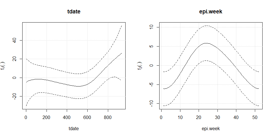
plot(mod2)
To perform diagnostic and influence analyses, execute:
aplms.diag.plot(mod2)
and
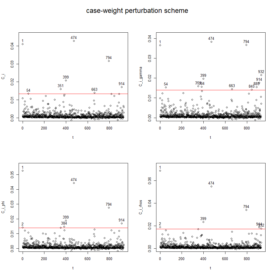
influenceplot.aplms(mod2, perturbation = c("case-weight"))